Algorithms
This page describes some details on the algorithms. Mainly the image reconstruction algorithms and priors, but also on the different subset types. Note that listmode cases apply to any custom detector reconstructions.
Note that https://github.com/villekf/OMEGA/wiki/Function-help#reconstruction-algorithms is also largely valid, though it lacks newer algorithms.
Subset types
The concept of subsets means that the measurement data is divided into N segments that are then reconstructed individually, as a sort of “sub-iterations”. This means that the reconstruction process is, usually, otherwise quite identical, but only a subset of
the measurement data is used to reconstruct the current estimate. The exact behavior of subset-based reconstruction depends on the selected algorithm. There are a total of 12 different ways to select subsets. Note that these apply only in the case that
you use subsets (subsets > 1). These are numbered from 0 to 11. In general, types 1-7 are more suitable for PET and 8-11 for CT and SPECT, while 0 is good for list-mode data.
Below is a short description for each and when to use each: In MATLAB/Octave use options.subset_type to specify the type and in Python options.subsetType. For example options.subset_type = 1 would use type 1. Type 8 is always used as the default.
Type 0
Type 0 is intended only for custom detector reconstructions, i.e. listmode cases. If you input your own source-detector coordinates or use the index-based reconstruction, then this is a viable subset method. Type 0 divides the data into NumberOfSubsets segments. For example, if you have 100 measurements and 4 subsets, the first subset will have measurements 1-25 (one-based indexing), next (26-50), third (51-75) and the last (76-100). This is useful if the measurement data is already “unordered” such as with listmode data. If, however, your data is ordered, i.e. for example the first 300 measurements are from ring 1, next 300 from ring 2, etc., then this method is not recommended.
Type 1
Type 1 divides the measurements by taking every Nth column measurement, i.e. if you have a 2D sinogram of size 10x20 and you use four subsets, then the first one will have measurements 1, 5, and 9 from the first column, 1, 5, and 9 from the second column, etc. Second subset will have measurements 2, 6, and 10 from the first column, 2, 6, and 10 from the second column, etc. The third subset measurements 3, 7 from the first column, 3, and 7 from the second column, etc. While 2D or 3D shape is assumed, this works for 1D inputs as well, i.e. listmode data. With 1D cases, it is assumed that only one column exists. Note that the order is always identical for each column.
Type 2
Same as above, but for every Nth row measurement. Unlike above, this requires 2D or 3D input to work. This type is not recommended! Does not work with listmode data.
Type 3
Selects the subsets randomly. Type 3 will randomly select the measurements for each subset. Works for all data types, but can be slower than any other subset type. Not recommended for CT. Works for listmode data as well.
Each subset has unique measurements, and as such there are no repetitions.
Type 4
Takes every Nth column. Type 4 requires 2D or 3D data and is similar to type 1, but instead of taking every Nth measurement along each column, type 4 takes all the measurements along the column. If you want to use measurement-based filtering with PET data, this method is recommended. It is also generally as good choice as type 1 for PET data. Does not support listmode data.
Type 5
Same as above but for rows. Not recommended method!
Type 6
Uses N number of angles to form each subset. First, the LORs are sorted according to the angle they create with the (positive) x-axis. Then n_angles angles are grouped together to form one subset. E.g. if n_angles = 2 then angles 0 and 1 form one subset, 2 and 3 another, etc. For 2D slices, there will be a total of 180°/nangles subsets and 360°/nangles for 3D.
This method is not recommended!
This method is based on: https://doi.org/10.1088/0031-9155/55/10/009
Type 7
Uses golden angle sampling to select the subsets. Each sinogram uses the same number of angles and the same angles, the golden angle sampling is thus performed on single sinogram basis. The next angle is selected such that the difference is roughly the same as the golden angle (approx. 111.246°). Currently this subset sampling is supported only by sinogram data.
Type 8
Type 8, and all the ones later, operate on full sinograms/projection images. Type 8 selects every Nth sinogram/projection for each subset. As such, this is mainly recommended for CT and SPECT. For PET, this method can be unreliable.
Listmode reconstruction is not supported.
Type 9
Selects the sinograms/projections randomly for each subset. Each subset has unique sinograms/projections. Mainly recommended for CT and SPECT. For PET, this method can be unreliable. Listmode reconstruction is not supported.
Type 10
Similarly to type 7, type 10 uses a golden angle-based selection. However, this time full projection images are used. As such, this only works for CT and SPECT and is also recommended mainly for 360 degree scans, though 180 should work too. Does not work with PET data. Listmode reconstruction is not supported.
Type 11
Uses prime factor sampling to select the projections/sinograms. Mainly recommended for CT and SPECT. For PET, this method can be unreliable. Listmode reconstruction is not supported.
Based on: https://doi.org/10.1109/42.241889
Stochastic subset selection
By default, the subsets are always used in the same order. However, it is now possible to also select the subsets randomly, though it is not completely random. The subsets are considered as “groups” that contain a set number of measurements, projections, or sinograms. The contents of these groups remain the same even if you use the stochastic subset selection, but the groups themselves are picked randomly. For example, if we have three subsets and 9 measurements, then subset 1 always contains the same three measurement, such as 1, 4, and 7. However, instead of using first subset 1, then subset 2, and lastly subset 3, any subset can be used first, second, etc. This means that while a group uses the same indices, the indices themselves are random.
You can enable the stochastic subset selection by setting options.stochasticSubsetSelection = true (or True in Python). The default is false.
Reconstruction algorithms
There are mainly two different types of algorithms: Poisson-based and least-squares based. Both also have variations that enable regularization. Below is a list of the algorithms and whether they are supported by a specific modality. EM refers to emission tomography as many Poisson-based algorithms have different variations for EM and transmission tomography. For transmission tomography versions, see the technical document (soon to be published).
To enable any algorithm, set the parameter defined below (usually their abbreviation) to true in MATLAB/Octave and to True in Python. Note that only one algorithm can be enabled at a time!
When in doubt, use PDHG, possibly with a measurement-based filtering preconditioner.
FDK/FBP
Full name: Feldkamp-Davis-Kress/Filtered backprojection algorithm
Enable with options.FDK.
Simple filtered backprojection. Scaling is currently incorrect for PET and SPECT data (CT should be fine) and as such the numerical values are not comparable to iterative methods. However, the image itself looks fine. GPU-based algorithm only. Useful for testing purposes, as it is a very fast method. Also useful for very high-dimensional µCT data.
For FDK reconstructions, you can optionally enable Parker weighting. By default this is off in all cases at the moment, but you can enable it by setting options.useParkerWeights to true. This method also allows additional tuning with the “q” parameter present in the original article
(see below). This is defined by options.ParkerWeight and is 0.25 by default. Using 1 enables the “original” Parker weights. Parker weighting can potentially improve the HU-value accuracy and improve image quality.
MLEM/OSEM
Full name(s): Maximum-likelihood expectation maximization/ordered subsets expectation maximization
Enable with options.OSEM.
While only OSEM is selectable, MLEM is enabled if no subsets are used (=``options.subsets = 1``). This method can be used for PET, SPECT or CT data, or any other Poisson-based data. Note that CT uses its own transmission tomography based formula, while PET and SPECT use the linear model. Useful algorithm for PET and SPECT, but not particularly recommended for CT. Use OSL_OSEM for the regularized version (see below).
RAMLA
Full name(s): Row-action maximum likelihood algorithm
Enable with options.RAMLA.
Similar to OSEM, but has guaranteed convergence and is dependent on the relaxation parameter options.lambda (or options.lambdaN in Python), see RELAXATION PARAMETER in the examples.
Slower to converge than OSEM. Can be used with or without subsets. Note that the default lambda values might not work with RAMLA. The default relaxation parameters are computed if the number of relaxation parameters doesn’t equal
the number of iterations, if the variable is omitted or if it’s zero. If you wish to enter your own relaxation parameters, make sure that the number of relaxation values equals the number of iterations!
Not recommended for CT but has transmission tomography based version implemented. See BSREM for regularized version.
Internally, the relaxation parameters are computed as follows:
if options.stochasticSubsetSelection
        for i = 1 : options.Niter
                lambda(i) = 1 / (0.4/options.subsets * i + 1);
        end
else
        for i = 1 : options.Niter
                lambda(i) = 1 / ((i - 1)/20 + 1);
        end
end
For CT, the values are further divided by 10000.
ET version based on: https://doi.org/10.1109/42.538946
MRAMLA
Full name(s): Modified Row-action maximum-likelihood algorithm
Enable with options.MRAMLA.
Unregularized version of the MBSREM. Almost identical to RAMLA, i.e. requires lambda (see above), but supports preconditioners. EM preconditioner is also highly recommended! Has some additional steps to guarantee convergence.
Also has a dedicated transmission tomography version. Useful for any Poisson-based data, if regularization is not used. The upper bound (see the article) can be optionally set with options.U, if zero, a default value is computed.
ET version based on: https://doi.org/10.1109/TMI.2003.812251
ROSEM
Full name(s): Relaxed ordered subsets expectation maximization
Enable with options.ROSEM.
Identical to OSEM except that it also includes relaxation (lambda, see RAMLA above) as well. Useful for testing/comparison purposes only. See ROSEM-MAP for the regularized version.
RBI
Full name(s): Rescaled block-iterative algorithm
Enable with options.RBI.
Subset-based algorithm similar to OSEM. Convergence is not guaranteed. No transmission tomography version. Useful for testing/comparison purposes only. See OSL-RBI for the regularized version.
Based on: https://doi.org/10.1109/83.499919
DRAMA
Full name(s): Dynamic row-action maximum likelihood algorithm
Enable with options.DRAMA.
Modified version of RAMLA. Requires some additional parameter tuning (see DRAMA PROPERTIES in the examples and the original article for details on the parameters), but can provide faster convergence. No transmission tomography version. No regularized version available.
COSEM
Full name(s): Complete-data ordered subsets expectation maximization
Enable with options.COSEM.
Unlike OSEM, has guaranteed convergence but is much slower to converge. No transmission tomography version. It is recommended to use ECOSEM or ACOSEM instead. Regularized version available with OSL-COSEM.
Based on: https://doi.org/10.1117/12.467144
ECOSEM
Full name(s): Enhanced complete-data ordered subsets expectation maximization
Enable with options.ECOSEM.
Uses both OSEM and COSEM to compute a converged version. Faster than regular COSEM. ACOSEM probably provides faster convergence. No transmission tomography version. Note that the “weighting” between COSEM and OSEM is identical to that of the original article!
ACOSEM
Full name(s): Accelerated complete-data ordered subsets expectation maximization
Enable with options.ACOSEM.
Accelerated version of COSEM. No transmission tomography version. Useful for non-regularized PET/SPECT reconstructions if convergence is required. Regularized version available with OSL-COSEM. Requires the acceleration parameter, see
ACOSEM PROPERTIES in the examples. The acceleration parameter is defined by options.h where 2 is the default value.
FISTA
Full name(s): Fast iterative shrinkage-threshold algorithm
Enable with options.FISTA.
Least-squares based algorithm. Can be used for any data and with or without subsets. Supports preconditioners. Does not support regularization at the moment (except the below one). Requires the computation of the Lipschitz
constant for the system. This is computed automatically if options.tauCP is omitted or zero, but a precomputed value can be input as well in which case the precomputation is omitted (this speeds up the reconstruction).
See PDHG PROPERTIES in the examples (the tauCP-values affect FISTA as well, this includes tauCPFilt if the filtering-based preconditioner is used).
Based on: https://doi.org/10.1137/080716542
FISTAL1
Full name(s): Fast iterative shrinkage-threshold algorithm with L1 regularization
Enable with options.FISTAL1.
FISTA with built-in L1 regularization. Otherwise identical to FISTA. Use options.beta as the regularization parameter.
LSQR
Full name(s): Least-squares
Enable with options.LSQR.
Least-squares based algorithm. Does not support subsets! Can be used for any data. Does not support regularization. Potentially useful test algorithm for CT data.
Based on: https://doi.org/10.1145/355984.355989
CGLS
Full name(s): Conjugate gradient least-squares
Enable with options.CGLS.
Least-squares based algorithm. Does not support subsets! Can be used for any data. Does not support regularization. Potentially useful test algorithm for CT data.
Based on: https://doi.org/10.6028/jres.049.044
SART
Full name(s): Simultanous algebraic reconstruction technique
Enable with options.SART.
Can be used with or without subsets. Uses same relaxation parameter as all the other algorithms using relaxation (i.e. options.lambda or options.lambdaN,see RAMLA above for some details).
None of the examples currently include this algorithm, but you can enable it with options.SART = true in MATLAB/Octave and options.SART = True in Python.
Supports regularization. Potentially useful test algorithm for CT data. Implementation 2 only! Use options.beta as the regularization parameter.
Based on: https://doi.org/10.1016/0161-7346(84)90008-7 and https://content.iospress.com/articles/journal-of-x-ray-science-and-technology/xst00110 and https://doi.org/10.1137/S089547980138705X
OSL-OSEM
Full name(s): One-step-late ordered subsets expectation maximization
Enable with options.OSL_OSEM.
OSL version of OSEM. Otherwise identical to OSEM but allows the use of regularization. MLEM version can be enabled by using only 1 subset. Everything that applies to OSEM/MLEM, applies here.
Use options.beta as the regularization parameter.
OSL based on: https://doi.org/10.1109/42.52985
MBSREM
Full name(s): Modified block-sequential regularized expectation maximization
Enable with options.MBSREM.
Regularized version of MRAMLA. Requires relaxation parameter lambda (see RAMLA for details), and supports preconditioners. EM preconditioner is also highly recommended! Has some additional steps to guarantee convergence.
Also has dedicated transmission tomography version. Useful for any Poisson-based data, if regularization is used. Use options.beta as the regularization parameter.
ET version based on: https://doi.org/10.1109/TMI.2003.812251
BSREM
Full name(s): Block-sequential regularized expectation maximization
Enable with options.BSREM.
Regularized version of RAMLA. However, unlike MBSREM, BSREM handles the regularization differently. While MBSREM computes the regularization after every subset, BSREM does it only after one full iteration (epoch). This can
sometimes be useful as less regularization steps might be used. Requires the relaxation parameter lambda. Also has a dedicated transmission tomography version. Use options.beta as the regularization parameter.
ET version based on: https://doi.org/10.1109/42.921477
ROSEM-MAP
Full name(s): Relaxed OSEM with maximum a posteriori
Enable with options.ROSEM_MAP.
Regularized version of ROSEM. Also like BSREM, this performs regularization at full iteration (epoch) level. Requires the relaxation parameter lambda (see RAMLA for details). Also has a dedicated transmission tomography version.
Use options.beta as the regularization parameter.
OSL-RBI
Full name(s): One-step-late RBI
Enable with options.OSL_RBI.
Regularized version of RBI. Otherwise identical. No transmission tomography version. Use options.beta as the regularization parameter.
OSL-COSEM
Full name(s): One-step-late COSEM
Enable with options.OSL_COSEM, see further details below.
Regularized version of either COSEM or ACOSEM. If options.OSL_COSEM = 1 then OSL-ACOSEM is used. With options.OSL_COSEM = 2 OSL-COSEM is used. ECOSEM is not supported.
Functions otherwise the same as their parent algorithms, so see those for some more details. No support for transmission tomography. Use options.beta as the regularization parameter.
PKMA
Full name(s): Preconditioned Krasnoselskii-Mann algorithm
Enable with options.PKMA.
Similar to MBSREM. Can be used without regularization but also supports regularization. Supports also proximal priors (TV and TGV). Supports preconditioners. Transmission tomography support. Requires the relaxation parameter lambda,
see RELAXATION PARAMETER in the examples and RAMLA above.
Useful for any Poisson-based data, if regularization is used. Useful also without regularization. The recommended algorithm for Poisson-based reconstructions. Unlike MBSREM, also requires the momentum parameter, see PKMA PROPERTIES in the examples.
The momentum parameter is defined in options.alpha_PKMA and if left zero or empty, it is computed automatically. You can instead input your own values, but make sure that the number of elements equals number of subsets * number of iterations!
If the values are computed automatically, these values can be adjusted with options.rho_PKMA and options.delta_PKMA. The automatic formula is (options.subsets is the number of subsets):
oo = 1;
for kk = 1 : options.Niter
        for ll = 0 : options.subsets - 1
                options.alpha_PKMA(oo) = 1 + (options.rho_PKMA *((kk - 1) * options.subsets + ll)) / ((kk - 1) * options.subsets + ll + options.delta_PKMA);
                oo = oo + 1;
        end
end
Note that for PET and SPECT data the relaxation parameter can safely begin at 1, but for CT data this is not the case. Due to this, PKMA is a bit difficult algorithm for CT data as you might need to manually adjust the relaxation parameter until it is of the right magnitude. Too high values will cause quick divergence, while too low values will cause slow convergence. For CT, the default value of 1 is divided by 10000 (when you use the default values). This should work for most CT applications, but it might not be optimal. To fix this, a proper normalization would be required for the backprojection (suggestions are welcome!).
ET version based on: https://doi.org/10.1109/TMI.2019.2898271
PDHG
Full name(s): Prima-dual hybrid gradient
Enable with options.PDHG.
PDHG refers to the L2 norm least-squares PDHG. Supports subsets, linear models, regularization, and preconditioners. Useful for any data. Measurement-based preconditioners are guaranteed to work unlike with PKMA or MBSREM.
By default, the primal and dual step-sizes are computed automatically, you can, however, input manual values too, see PDHG PROPERTIES in the examples. Supports also adaptive step-size computations, but it is not recommended with multi-resolution
reconstruction. Supports both proximal priors as well as regular non-linear convex ones (in the latter case it is actually the Condat-Vu algorithm).
The primal value is set with options.tauCP, but is computed automatically if empty or zero. If using a filtering-based preconditioner, a specific primal value is set with options.tauCPFilt, and like the previous one, is computed automatically
if zero or empty. Dual value is set with options.sigmaCP, but 1 can be safely used. Update step-size is set with options.thetaCP, but can also be safely set as 1.
The primal and dual variables can also be updated adaptively by setting options.PDAdaptiveType to either 1 or 2. Note that 1 corresponds to rule B from the article and 2 to rule A. See the article for details.
CV
Full name(s): Condat-Vu
Enable with options.PDHG.
Exactly the same as above PDHG, but for convex gradient-based priors. CV is basically used whenever gradient-based regularizers are used.
PDHGL1
Full name(s): Prima-dual hybrid gradient with L1 minimization
Enable with options.PDHGL1.
Same as above but with L1 norm. Has exactly the same properties as the L2 norm version.
PDHGKL
Full name(s): Prima-dual hybrid gradient with Kullback-Leibler divergence
Enable with options.PDHGKL.
Same as above but for Kullback-Leibler divergence. This is useful only for linear Poisson-based data, e.g. PET or SPECT. Otherwise has the same properties as the L2 norm one.
PDDY
Full name(s): Primal-dual Davis-Yin
Enable with options.PDDY.
Variation of PDHG L2 norm version. Is not as strict with the requirements for primal and dual step-sizes with non-linear regularizers. Recommended only if PDHG fails with some specific prior, but that should not happen with built-in priors. Slightly slower than PDHG but otherwise everything is identical.
ASD-POCS
Full name(s): ASD - Projection onto convex sets
Enable with options.ASD_POCS.
Currently not included in any of the examples, but you can enable it with options.ASD_POCS = true (MATLAB/Octave) or options.ASD_POCS = True (Python). Adjustable parameters are options.POCS_NgradIter
(number of iterations for the denoising phase), options.POCS_alpha, options.POCS_rMax, options.POCS_alphaRed and options.POCSepps. Note that options.POCSepps is the epsilon value in the original article.
All values have default values, which are taken from the original article, except for epsilon value which is 1e-4. Supports subsets, but doesn’t support any preconditioners. Note that, like SART, this algorithm requires
the relaxation parameters options.lambda (MATLAB/Octave) or options.lambdaN (Python), see RAMLA. You can use the default value(s) or input your own values. Implementation 2 only!
Unlike the original article, any non-proximal prior can be used here, though the functionality cannot be guaranteed!
Does not support projector type 6 at the moment.
SAGA
Full name(s): SAGA
Enable with options.SAGA.
Only included in the full examples, but can be enabled with options.SAGA = true (MATLAB/Octave) or options.SAGA = True (Python). Supports gradient-based regularization. Implementation 2 only! Supports both emission and transmission tomography.
Based on: https://arxiv.org/abs/1407.0202
FISTA acceleration
Not an algorithm but rather an acceleration method for algorithms. You can enable it with options.FISTA_acceleration = true (MATLAB/Octave) or options.FISTA_acceleration = True (Python). Can help with convergence speed
but can also cause artifacts in the reconstructions. Quality might be algorithm-dependent.
Priors
Many of the priors are dependent on the neighborhood size, i.e. the number of neighboring voxels that are taken into account during regularization. This can be selected for all three dimensions (X/Y/Z) though at the moment
X and Y should be identical (transaxial dimensions). For example, options.Ndx = 1, options.Ndy = 1, options.Ndz = 0 selects all the 8 neighboring transaxial voxels, while with options.Ndz = 1 a total of 27 voxels would
be included, etc. The larger the neighborhood, the longer the computation time. If a prior is NOT affected by this, it is specifically mentioned! The regularization strength can always be adjusted with options.beta.
As with algorithms, a regularizer can be selected by setting the specific regularizer to true or True (Python). Note that only some algorithms support regularizers, but this should be something the software checks beforehand.
Only one regularizer can be selected at a time!
Below is another example of the neighborhood. In the below (2D) example we have options.Ndx = 2 and options.Ndy = 2, with the center pixel in white and the neighborhood as blue. Note that the NLM patch region works the same way.
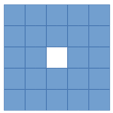
Example neighborhood with options.Ndx = 2 and options.Ndy = 2.
Quadratic
Full name(s): Quadratic prior
Enable with options.quad.
Simple quadratic prior. Define the weights at QP PROPERTIES (see the examples). By default, the distance of each voxel in the neighborhood from the center voxel is used as the weight, normalized such that the sum of the weights equals one. Custom weights can be input to options.weights.
The weight vector should be of size (Ndx*2+1) * (Ndy*2+1) * (Ndz*2+1) and the middle value inf.
Huber prior
Full name(s): Huber prior
Enable with options.Huber.
Similar to quadratic prior, but can prevent large variations and thus artifacts happening by limiting the values with options.huber_delta. See HP PROPERTIES in the examples. The weighting functions the same ways as quadratic prior, meaning that
you can input your own weights into options.weights_huber or leave it empty and use the default ones. By default, the distance of each voxel in the neighborhood from the center voxel is used as the weight, normalized such that the sum of the weights equals one.
The weight vector should be of size (Ndx*2+1) * (Ndy*2+1) * (Ndz*2+1) and the middle value inf, if custom values are input.
Based on: https://doi.org/10.1002/9780470434697
MRP
Full name(s): Median root prior
Enable with options.MRP.
Median root prior. By default, the prior uses normalization. Disabling this normalization, however, can lead to improvement in image quality. You can turn the normalization off with options.med_no_norm = true. Can be useful prior
with PET or SPECT data.
Based on: https://doi.org/10.1007/BF01728761
L-filter
Full name(s): L-filter
Enable with options.L.
Custom weights can be input, see L-FILTER PROPERTIES in the examples. The variable for entering the weights is options.a_L. The weight vector should be of size (Ndx*2+1) * (Ndy*2+1) * (Ndz*2+1) (middle value is NOT inf).
If custom weights are not given, the options.oneD_weights determines whether the 1D (true) or 2D (false) weighting scheme is used. In 1D case, if (Ndx*2+1) * (Ndy*2+1) * (Ndz*2+1) = 3, = 9 or = 25 then the weights are exactly as
in the literature. Otherwise the pattern follows a Laplace distribution. In the 2D case, the weights follow Laplace distribution, but are also weighted based on the distance of the neighboring voxel from the center voxel.
For the Laplace distribution, the mean value is set to 0 and b = 1/sqrt(2). The weights are normalized such that the sum equals 1.
Note: L-filter isn’t currently supported in Python!
FMH
Full name(s): Finite impulse response median hybrid
Enable with options.FMH.
Custom weights can be input into options.fmh_weights, see FMH PROPERTIES in the examples. The weight vector should be of size [Ndx*2+1, 4] if Nz = 1 or Ndz = 0 or [Ndx*2+1, 13] otherwise. The weight of the center pixel should also be the middle value when the weight matrix is in vector form.
The weights are normalized such that the sum equals 1.
If custom weights are not provided, then the options.fmh_center_weight parameter is needed. The default value is 4 as in the original article. The default weighting scheme is based on the distance from the center voxel and normalized such that the sum of the weights equals one.
Note: FMH isn’t currently supported in Python!
Weighted mean
Full name(s): Weighted mean
Enable with options.weighted.
The mean type can be selected as the arithmetic mean (options.mean_type = 1), harmonic mean (options.mean_type = 2) or geometric mean (options.mean_type = 3). See WEIGHTED MEAN PROPERTIES in the example.
Custom weights can be input to options.weighted_weights. The weight vector should be of size (Ndx*2+1) * (Ndy*2+1) * (Ndz*2+1).
If custom weights are not provided, then the options.weighted_center_weight parameter is needed. The default value is 4. The default weighting scheme is based on the distance from the center voxel, and normalized such that the sum of the weights equals one.
Based on: https://doi.org/10.1109/42.61759 and https://doi.org/10.1109/TMI.2002.806415
TV
Full name(s): Total variation, hyperbolic prior with anatomical weighting, total variation with anatomical weighting, weighted total variation, modified Lange prior
Enable with options.TV, for other types see below.
TV is not affected by the neighborhood size!
TV is “special” since it actually contains several different variations. See TV PROPERTIES in the examples for the parameters. Note that for proximal TV, see Proximal TV. This is the gradient-based TV.
First, is the “TV type”, options.TVtype. Types 1 and 2 are identical if no anatomical weighting is used. Type 3 is the hyperbolic prior if no anatomical weighting is used. Type 6 is a weighted TV prior. TV type 4 is the Lange prior.
Since this applies to the “gradient”-based TV, the smoothing term can be adjusted (options.TVsmoothing). This smoothing term should not be zero as it prevents division and square root by zero. Larger values lead to smoother images, but smaller values can
make the regularization unstable.
Anatomical weighting can be enabled with options.TV_use_anatomical. The reference image can be either a mat-file or a variable. In the former case, input the name and path to options.TV_reference_image, otherwise the variable.
If a mat-file is used, the reference image should be the only variable in the mat-file.
options.T is the edge threshold parameter in type 1, scale parameter for side information in type 2 and weight parameter for anatomical information in type 3.
options.C is the weight of the original image in type 3.
options.SATVPhi is the adjustable parameter of type 4 (Lange) or the strength of the weighting in type 6.
In the future, Lange will probably become a separate prior.
The recommended ones are types 1 or 4.
Proximal TV
Full name(s): Proximal total variation
Enable with options.ProxTV.
Proximal TV is not affected by the neighborhood size.
The proximal mapping version of TV. There are no adjustable parameters, and this only works with algorithms that support proximal methods (PKMA and PDHG and its variants).
Mathematically more correct version of TV.
Anisotropic Diffusion Median Root Prior
Full name(s): Anisotropic Diffusion Median Root Prior
Enable with options.AD.
In general, this prior is not recommended and is included merely for historical and experimental purposes.
It functions the same as median root prior, except that, rather than use median filtered image, it uses anisotropic diffusion filtered image.
All the adjustable parameters are from: https://arrayfire.org/docs/group__image__func__anisotropic__diffusion.htm
APLS
Full name(s): Asymmetric parallel level sets
Enable with options.APLS.
Based on: https://doi.org/10.1109/TMI.2016
Using asymmetric parallel level sets requires the use of anatomic prior. Without anatomical prior it functions as TV types 1 and 2.
Regularization parameters for all MAP-methods can be adjusted.
options.eta is a scaling parameter in regularized norm (see variable η in the reference).
options.APLSsmoothing is a “smoothing” parameter that also prevents zero in square root (it is summed to the square root values). Has the same function as the TVsmoothing parameter (see eq. 9 in the reference).
options.APLS_reference_image is the reference image itself OR name of the file containing the anatomical reference images (image size needs to be the same as the reconstructed images). The reference images need to be the only variable in the file.
Hyperbolic prior
Full name(s): Hyperbolic prior
Enable with options.hyperbolic.
Based on: https://doi.org/10.1109/83.551699 and https://doi.org/10.1088/0031-9155/60/6/2145
Modified hyperbolic prior, previously exclusively used as TV type 3. Unlike TV type 3, doesn’t support anatomic weighting.
options.hyperbolicDelta can be used to adjust the edge emphasizing strength.
TGV
Full name(s): Proximal total generalized variation
Enable with options.TGV.
TGV is not affected by the neighborhood size.
Based on: https://doi.org/10.1137/090769521
Recommended only for methods that support proximal mappings (PDHG and its variants, PKMA).
options.alpha0TGV is the first weighting value for the TGV (see parameter α1 in the reference).
options.alpha1TGV is the second weighting value for the TGV (see parameter α0 in the reference). Weight for the symmetrized derivative.
RDP
Full name(s): Relative difference prior
Enable with options.RDP.
Based on: https://doi.org/10.1109/TNS.2002.998681
RDP can be a bit confusing prior as there are 2/3 different ways it is computed. First of all, implementation 2 is highly recommended for RDP in MATLAB/Octave (Python only supports implementation 2). Second, with implementation 2 it is recommended to use the OpenCL or CUDA versions and not the CPU version.
RDP with implementation 2 (OpenCL + CUDA) has two different methods. The default is similar to the original RDP, i.e. only the voxels next to the current voxel are taken into account (voxels that share a side with the current voxel).
This means that options.Ndx/y/z are not used with the default method.
Second method is enabled by setting options.RDPIncludeCorners = true (options.RDPIncludeCorners = True for Python). This changes the functionality of the RDP significantly. First of all, the neighborhood size affects RDP
as well, i.e. the parameters options.Ndx/y/z. This second version thus uses square/rectangular/cubic neighborhoods. Second, the same weights are used as with quadratic prior, i.e. distance-based weights. You can input your own weights into options.weights or use the distance-based weights (the distance from the current voxel to
the neighborhood voxel) which is the default option. The default version (i.e. when options.RDPIncludeCorners = false) does not use any weighting. Lastly, this second version supports a “reference image” weighting, based on: https://dx.doi.org/10.1109/TMI.2019.2913889.
To enable you need to additionally set options.RDP_use_anatomical and provide the reference image either as mat-file in options.RDP_reference_image (MATLAB/Octave) or options.RDP_referenceImage (Python) or as a vector.
You need to manually compute the reference image. The reference image weighting itself is computed automatically, i.e. the kappa values.
When using RDP with implementation 2 and CPU, the functionality is the same as in the first, default, method. Second method is not available.
When using other implementations, the functionality is closer to the second method. However, no reference image weighting is supported.
In all cases, the edge weight can be adjusted with options.RDP_gamma.
GGMRF
Full name(s): Generalized Gaussian Markov random field
Enable with options.GGMRF.
Based on: https://doi.org/10.1118/1.2789499
The original article includes adjustable parameters p, q and c which can be adjusted with options.GGMRF_p, options.GGMRF_q, and options.GGMRF_c, respectively.
NLM
Full name(s): Non-local means, non-local total variation, non-local relative difference, non-local generalized Gaussian Markov random field, non-local Lange
Enable with options.NLM.
Based on: https://doi.org/10.1137/040616024
options.sigma is the filtering parameter/strength. Larger values smooth the image, while smaller ones emphasize edges/noise.
The patch region is controlled with parameters options.Nlx, options.Nly and options.Nlz. The similarity is investigated in this area and the area is formed just like the neighborhood.
The strength of the Gaussian weighting (standard deviation) can be adjusted with options.NLM_gauss, a value of 2 should work well in most cases.
If options.NLM_use_anatomical = true then an anatomical reference image is used in the similarity search of the neighborhood. Normally the original image is used for this. options.NLM_reference_image is either the reference image itself OR is the name of the anatomical reference data file. The reference images need to be the only variable in the file.
NLM, by default, uses the original NLM, but it can also use other potential functions in a non-local fashion. Setting any of the below ones to true, uses the corresponding method. Note that from the options below, select only one! All other NLM options affect the below selections as well.
If you wish to use non-local total variation, set options.NLTV = true.
NLM can also be used like MRP (and MRP-AD) where the median filtered image is replaced with NLM filtered image. This is achieved by setting options.NLM_MRP = true. This is computed without normalization ((λ - MNLM)/1).
Non-local relative difference prior can se selected with options.NLRD = true. Note that options.RDP_gamma affects NLRD as well, see RDP.
Non-local generalized Gaussian Markov random field prior can be selected with options.NLGGMRF = true. As with RDP, the p, q, and c parameters affect this prior as well, see GGMRF.
Non-local Lange function is enabled with options.NLLange. options.SATVPhi is the tuning parameter for the Lange function, see TV and specifically type 4.
All the non-local methods also support an “adaptive” non-local weighting. This is enabled with options.NLAdaptive and is based on http://dx.doi.org/10.1016/j.compmedimag.2015.02.008. Note that the filter parameter (options.sigma)
is the s value from the paper, while the t value is adjusted with options.NLAdaptiveConstant.
Preconditioners
The use of preconditioners is slightly easier in Python than in MATLAB/Octave. This is because in MATLAB/Octave you need to input the whole vector that specifies the selected preconditioners, in Python you only need to set the desired one to True.
All preconditioners are off by default.
Note
Most of the preconditioners are supported as-is only with built-in algorithms. However, the filtering-based measurement-based preconditioner has been implemented as a separate MATLAB/Python function. Some of the preconditioners are also easy to compute manually.
Image-based preconditioners
For image-based preconditioners, in MATLAB/Octave you need to input options.precondTypeImage = [false;false;false;false;false;false;false]; and then select the appropriate preconditioners by setting its element to true. See below for the elements.
In general you can select multiple preconditioners, except for diagonal, EM and IEM preconditioners, which are mutually exclusive. Image-based preconditioners, as the name implies, work in the image-space.
Only certain algorithms support image-based preconditioners. These are: MRAMLA, MBSREM, FISTA, FISTAL1, PKMA, PDHG, PDHGKL, PDHGL1, PDDY, and SAGA. If an image-based preconditioner is used with an algorithm not listed, it’s not used.
Diagonal preconditioner
The diagonal preconditioner is simply the inverse of the image-based sensitivity image, i.e. 1/(A^T1).
In MATLAB/Octave, options.precondTypeImage = [true;false;false;false;false;false;false]; enables this preconditioner. For Python, you can simply use options.precondTypeImage[0] = True. Note that this is mutually exclusive with EM and IEM preconditioners!
This means that you can only select one of these! You can also select some of the other preconditioners though.
EM preconditioner
Similar to above, but the previous estimate f is included as well f/(A^T1).
In MATLAB/Octave, options.precondTypeImage = [false;true;false;false;false;false;false]; enables this preconditioner. For Python, you can simply use options.precondTypeImage[1] = True. Note that this is mutually exclusive with diagonal and IEM preconditioners!
This means that you can only select one of these! You can also select some of the other preconditioners though.
IEM preconditioner
Based on: https://doi.org/10.1109/TMI.2019.2898271
Similar to above, but a reference image is needed: max(f, fRef, epsilon)/(A^T1). epsilon is a small value to prevent too small values. You need to input the reference image beforehand to options.referenceImage.
In MATLAB/Octave, options.precondTypeImage = [false;false;true;false;false;false;false]; enables this preconditioner. For Python, you can simply use options.precondTypeImage[2] = True. Note that this is mutually exclusive with diagonal and EM preconditioners!
This means that you can only select one of these! You can also select some of the other preconditioners though.
Momentum-like preconditioner
Essentially a subset-based relaxation. Based on: https://doi.org/10.1109/TMI.2022.3181813
You can input the momentum parameters with options.alphaPrecond or let OMEGA compute parameters with same logic as with PKMA by inputting options.rhoPrecond and options.delta1Precond. If these values are omitted, the PKMA variables are used
instead. The “formula” for computing the default ones is the same as with PKMA, see that section for details.
In MATLAB/Octave, options.precondTypeImage = [false;false;false;true;false;false;false]; enables this preconditioner. For Python, you can simply use options.precondTypeImage[3] = True.
Gradient-based preconditioner
Uses a weighted gradient of the current estimate as a preconditioner. Based on: https://doi.org/10.1109/TMI.2022.3181813
You need to specify the iteration in which the preconditioner is first computed with options.gradInitIter. It is not recommended to use the first iteration due to the blurry estimate. Then you need to specify the last iteration
where the gradient is computed with options.gradLastIter. The gradient is no longer computed after this iteration, but the last computed gradient is still used in all the remaining iterations.
You also need to specify the lower and upper bound values with options.gradV1 and options.gradV2. See the paper for details.
Can improve convergence if properly configured, but can be difficult and time-consuming to get working properly. Also increases the computation time due to the need to compute the gradient of the estimate.
In MATLAB/Octave, options.precondTypeImage = [false;false;false;false;true;false;false]; enables this preconditioner. For Python, you can simply use options.precondTypeImage[4] = True.
Filtering-based preconditioner
This preconditioner is not particularly recommended. If possible, the measurement-based filtering preconditioner should be used instead. The behavior is very similar to that of the measurement-based one (see below), but
the filtering is instead applied to the backprojection. This, however, tends to make the reconstruction quite unstable and usually filters the image too much. Currently, there is no particular way to adjust the filtering
amount except to try other windows. For this, the Gaussian window (options.filterWindow = 'gaussian') is probably the best as you can adjust the strength of the filtering with options.normalFilterSigma. The cut-off
frequency can be adjusted, if necessary, with options.cutoffFrequency. Available windows are: hamming, hann, blackman, nuttal, parzen, cosine, gaussian, shepp-logan and none.
In MATLAB/Octave, options.precondTypeImage = [false;false;false;false;false;true;false]; enables this preconditioner. For Python, you can simply use options.precondTypeImage[5] = True.
Curvature-based preconditioner
Based on: https://doi.org/10.1109/TMI.2003.812251
This is specifically based on equation (26) from the original article. Note that regularization is NOT taken into account even if selected.
In MATLAB/Octave, options.precondTypeImage = [false;false;false;false;false;false;true]; enables this preconditioner. For Python, you can simply use options.precondTypeImage[6] = True.
Measurement-based preconditioners
For measurement-based preconditioners, in MATLAB/Octave you need to input options.precondTypeMeas = [false;false]; and then select the appropriate preconditioners by setting its element to true. See below for the elements.
Measurement-based preconditioners, as the name implies, work in the measurement-space.
Only certain algorithms support measurement-based preconditioners. These are: MRAMLA, MBSREM, FISTA, FISTAL1, PKMA, PDHG, PDHGKL, PDHGL1, PDDY, and SAGA. If a measurement-based preconditioner is used with an algorithm not listed, it’s not used.
Diagonal preconditioner
The diagonal preconditioner is simply the inverse of measurement-based sensitivity image, i.e. 1/(A1).
In MATLAB/Octave, options.precondTypeMeas = [true;false]; enables this preconditioner. For Python, you can simply use options.precondTypeMeas[0] = True.
Filtering-based preconditioner
Based on: https://doi.org/10.1007/s10851-025-01276-4
This preconditioner applies a high-pass filtering to the forward projection. The behavior can be slightly different depending on the algorithm. For example, PDHG, and its variants, use a special reconstruction method when this preconditioner
is selected. The convergence of PDHG, and its variants, are also guaranteed with this preconditioner. This should also work fine with FISTA, but other algorithms may or may not work optimally. Since this preconditioner emphasizes high-frequency
regions, it can also emphasize noise faster than contrast. Due to this, it can be beneficial to use this filtering in N initial iterations and then turn it off. This is possible by modifying options.filteringIterations. Note that this
includes subiterations (subsets) as well so if you want to turn off the filtering after 2 iterations and you have in total 5 iterations with 20 subsets, then you should set options.filteringIterations = 40. You can also turn off the filtering
in the middle of subiterations. The functionality of this preconditioner is very similar to that of the filtered backprojection or FDK, but it is instead applies as a preconditioner. By default, the preconditioner uses Hamming windowing, but other
types of windows are also available: hamming, hann, blackman, nuttal, parzen, cosine, gaussian, shepp-logan and none (e.g. options.filterWindow = 'hann'). The cut-off
frequency can be adjusted, if necessary, with options.cutoffFrequency.
In CT, it is highly recommended to include this preconditioner as it significantly speeds up the reconstructions. It also works for other modalities, though TOF-PET data might not see any benefit.
In MATLAB/Octave, options.precondTypeMeas = [false;true]; enables this preconditioner (while turning off the diagonal preconditioner). For Python, you can simply use options.precondTypeMeas[1] = True.