Data/artifact corrections
This page describes some details on the different data/artifact correction methods available in OMEGA. Available are: randoms, scatter, attenuation, normalization, out-of-FOV, and offset corrections.
Randoms correction
This is PET only feature. The randoms correction data can be either included in the reconstructions in an “ordinary Poisson” (OP) way, or precorrected. For OP, you must select options.corrections_during_reconstruction = true
before running the reconstructions. As for the randoms corrections data, you can input it manually into options.SinDelayd variable, have them automatically loaded if using GATE, Inveon or Biograph data with randoms data, or
input a mat-file containing only the randoms data when prompted. If precorrection is used, then the randoms are simply subtracted from the measurement data. Note that you can also use precorrection yourself manually, but in such
a case you should set randoms correction as false.
You can also select variance reduction (options.variance_reduction) and/or smoothing (options.randoms_smoothing) for the randoms data. Note that these features are not yet available on Python. The former performs variance
reduction to the randoms data, while latter uses 8x8 moving mean smoothing. The mean-size can be adjusted by manually modifying the randoms_smoothing function.
See https://doi.org/10.1088/0031-9155/44/4/010 for details on variance reduction.
Scatter correction
Scatter correction data cannot be created with OMEGA at the moment, though you can extract GATE scatter data from PET simulations. However, you can add your own scatter correction data by inputting it into options.ScatterC
variable. Same variance reduction (options.scatter_variance_reduction) and smoothing operations (options.scatter_smoothing) can be applied to the scatter data as well. You can also normalize PET scatter data with
options.normalize_scatter if you use normalization correction.
Attenuation correction
This is PET and SPECT only feature. Adjust the state of the correction with options.attenuation_correction. The attenuation data HAS to be input by the user. Two different attenuation data are accepted: images and sinograms.
This means that the correction can be applied either by using attenuation images or by using attenuation sinograms. Note that for the attenuation images, the images HAVE to be scaled to the corresponding energy! Default is attenuation
images, but this can be adjusted with options.CT_attenuation, where false uses sinograms. Input the, preferable full, path of the attenuation data into options.attenuation_datafile. If your attenuation data is oriented
different to the reconstruction, you can rotate the attenuation image with options.rotateAttImage, where the image is rotated as N * 90 degress, where N = options.rotateAttImage. Similarly you can also flip the transaxial and/or
axial directions with options.flipAttImageXY and options.flipAttImageZ, respectively. Note that the attenuation image also has to have the same dimensions as the output image.
For GATE data, the attenuation images created by MuMap actor can be used.
Note that the units in OMEGA are in millimeters!
Normalization correction
This is PET only feature and enabled with options.normalization_correction. There are two options, either you can input precomputed normalization correction sinogram or then you can use a specific normalization measurement
and compute the normalization coefficients with OMEGA. For the latter, set options.compute_normalization to true and select the desired normalization components with options.normalization_options. Normalization correction
components to include (1 means that the component is included, 0 that it is not included). First: Axial geometric correction, Second: Detector efficiency correction, Third: Block profile correction, Fourth: Transaxial geometric
correction (NOT recommended when using normalization data that does not encompass the entire FOV). E.g. [1 1 0 0] computes normalization correction for axial geometric effects and detector efficiency. If a cylinder was used for
the normalization measurements that is smaller than the FOV, you can input its radius with options.normalization_phantom_radius. This is used for automatic attenuation correction. If you input the radius, you also need to input
the attenuation coefficient of the material with options.normalization_attenuation. You can also use automatic scatter correction with options.normalization_scatter_correction. Note that Python does not (yet) support computing of
the normalization coefficients.
If you use normalization data NOT computed by OMEGA, you need to set options.use_user_normalization to true. To insert the normalization coefficient data, either input the data into options.normalization or select it when running the code
and getting the prompt for the data. The normalization data has to be either nrm-file (Inveon normalization) or mat-file (has to be the only variable, or at least the first variable). Normalization data computed with OMEGA are saved
to the mat-files folder and loaded automatically if the same measurement dimensions and scanner are used.
For details on the component-based normalization, see for example https://doi.org/10.1088/0031-9155/43/1/012
Out-of-FOV correction
This is mainly for CT, but might work with other modalities as well. Out-of-FOV correction aims to correct artifacts caused by attenuating material outside of the active FOV, see the below figure for an example.
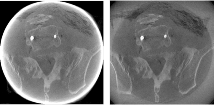
Left: No correction. Right: Projection extrapolation and extended FOV with multi-resolution.
This correction is a bit more complicated than the other ones as there isn’t a single option to turn on. There are two main options, projection extrapolation and extended FOV. For the projection extrapolation, the projection images
can be extrapolated in the transaxial and/or axial directions, essentially top/bottom and left/right. Default extrapolation length is 20% (0.2) of the original size per direction, but this can be optionally adjusted with options.extrapLength.
The extrapolation is simple next/previous extrapolation, i.e. depending on the side either the previous or next value is used. The extrapolated data is then scaled logarithmically such that the very edge is air and the values scale
towards this air value. Note that this step involves linearization of the data and then transforming it back into Poisson-based count data which can cause some numerical inaccuracy to the extrapolated regions. The original data
is not affected by this. You can separately select the transaxial and axial extrapolations with options.transaxialExtrapolation and options.axialExtrapolation, respectively. Extrapolation itself is enabled with
options.useExtrapolation.
In addition to, or alternatively, you can use extended FOV. This simply extends the FOV, but does have some additional advantages to doing this manually. First, the image is automatically cropped to the original size, second
regularization is generally only applied to the main FOV and third, you can select multi-resolution reconstruction. As with extrapolation, the extended FOV can be applied only to transaxial direction (XY) and/or axial direction (Z) with
options.transaxialEFOV and options.axialEFOV, respectively. You can enable extended FOV with options.useEFOV. Normally, the extended FOV uses the same voxel size, but you can use increased voxel size with the multi-resolution
reconstruction, enabled with options.useMultiResolutionVolumes. The extended volume is divided into separate volumes, where the amount depends on whether transaxial and/or axial directions are included. If both are included, there
will be 6 multi-resolution volumes plus the main volume. The multi-resolution volumes can have larger voxel size than the main volume. This can be controlled with options.multiResolutionScale, where the default value of 1/4 means
that the original size is divided by this value, i.e. the resolution is 1/4 of the original and the voxel size four times larger. The default extended FOV extension length is 40% (0.4) of the original size per side. With 1/4 scale, this is
essentially reduced to 10% increase in voxel count. You can adjust this manually with options.eFOVLength. With multi-resolution volumes, the mask image and regularization are only used for the main volume!
See https://doi.org/10.1088/1361-6560/aa52b8 for details on the multi-resolution method. Note that the OMEGA implementation may not exactly match the paper.
See https://dx.doi.org/10.1118/1.1776673 for another example of projection extrapolation.
Offset correction
This is CT only feature and can be enabled with options.offsetCorrection. If you have an offset imaging case, setting this to true should remove any offset artifacts. This is often called redundancy weighting. The weighting should
be done automatically.
Examples of offset papers include https://dx.doi.org/10.1109/nssmic.2010.5874179 and https://dx.doi.org/10.1088/0031-9155/58/2/205 and https://dx.doi.org/10.1118/1.1489043 and https://dx.doi.org/10.1088/1361-6560/ac16bc. Note that although they present different weights, the results are the same.