Data/artifact corrections
This page describes details of the different data/artifact correction methods available in OMEGA. Available methods are: arc, randoms, scatter, attenuation, normalization, out-of-FOV, and offset corrections.
While this is highlighted in the section below, it is important to note that if you input your own data in Python, you need to make sure the data is Fortran-ordered!
Arc correction
This is a PET-only feature. In general, it is not recommended to use arc correction, but with certain scanners it can help reduce aliasing artifacts with single ray-based projectors. It can be enabled with options.arc_correction.
Internally, arc correction uses the MATLAB function scatteredInterpolant to interpolate the sinograms. If that function is not available, griddata is used instead. In Python, SciPy’s griddata is always used.
Arc correction can be a slow process, but if you own the Distributed Computing Toolbox, that is automatically used and should speed up the process. For Python or Octave, however, there are no means to speed up the process.
You can control the interpolation type with options.arc_interpolation. The supported types are the same as those supported by scatteredInterpolant or griddata (MATLAB/Octave or Python).
The default type is linear.
From the first OMEGA article: In arc correction, the orthogonal distances between adjacent LORs with the same angle are made equidistant, as the circular configuration of most PET designs causes the adjacent LORs not to be equidistant. Using the original detector coordinates and the new detector coordinates of equidistant LORs, the sinogram is interpolated into this new detector grid. This procedure would be mandatory when using analytical methods such as FBP but is not required with iterative methods. However, since the measurement data becomes equally spaced, it can remove aliasing artifacts in certain cases (e.g. with Inveon data). As with randoms and normalization, the arc correction is a separate MATLAB/Octave function.
See https://doi.org/10.1117/12.618140 for more details on arc correction.
Note
Arc correction has not been tested much and will probably work well only with certain scanner configurations. In general, its use is not recommended.
Randoms correction
This is a PET-only feature. Randoms correction uses a previously obtained estimate of the randoms either as a precorrection or during the reconstruction.
The randoms correction data can be either included in the reconstructions in an “ordinary Poisson” (OP) way, or precorrected. For OP, you must select options.corrections_during_reconstruction = true
before running the reconstructions. As for the randoms corrections data, you can input it manually into the options.SinDelayd variable (in Python, you need to make sure the data is Fortran-ordered!), have them automatically loaded if using GATE,
Inveon, or Biograph data with randoms data, or input a mat-file containing only the randoms data when prompted. If precorrection is used, then the randoms are simply subtracted from the measurement data. Note that you can also apply precorrection
manually, but in such a case, you should set randoms correction to false.
You can also select variance reduction (options.variance_reduction) and/or smoothing (options.randoms_smoothing) for the randoms data. The former performs variance
reduction on the randoms data, while the latter uses 7x7 moving mean smoothing. The mean size can be adjusted by manually modifying the randoms_smoothing function.
See https://doi.org/10.1088/0031-9155/44/4/010 for details on variance reduction.
Note
For custom reconstructions using the projector operators, randoms has to be handled manually by the user.
Scatter correction
Scatter correction data cannot be created with OMEGA at the moment, but you can extract GATE scatter data from PET simulations (GATE 9.X or earlier). However, you can add your own scatter correction (estimate) data by inputting it into the options.ScatterC
variable. The same variance reduction (options.scatter_variance_reduction) and smoothing operations (options.scatter_smoothing) as with randoms can be applied to the scatter data as well. You can also normalize PET scatter data with
options.normalize_scatter if you use the normalization correction. In Python, you need to make sure that the data is Fortran-ordered!
By default, the scatter correction is either subtracted from the measurements (if precorrected) or added to the forward projection (if ordinary Poisson, i.e. options.corrections_during_reconstruction = true). However, it is possible to have
multiplicative scatter correction instead. In such a case, the scatter data is multiplied with the projector operators. To enable this, set options.subtract_scatter = false. Variance reduction, normalization, and/or smoothing should
not be used in this case. Otherwise, the process is similar, i.e. add the data into options.ScatterC.
Note
For custom reconstructions using the projector operators, scatter has to be handled manually by the user. The options.subtract_scatter = false case should work automatically, but this is untested.
Attenuation correction
This is a PET and SPECT-only feature. Adjust the state of the correction with options.attenuation_correction. The attenuation data HAS to be input by the user. Two different attenuation data are accepted: images and sinograms.
This means that the correction can be applied either by using attenuation images or by using attenuation sinograms. Note that for both cases, the images/sinograms HAVE to be scaled to the corresponding energy! The default is attenuation
images, but this can be adjusted with options.CT_attenuation, where false uses sinograms. Input the preferably full path of the attenuation data into options.attenuation_datafile OR input the attenuation data itself into options.vaimennus.
If your attenuation data is oriented
differently from the reconstruction, you can rotate the attenuation image with options.rotateAttImage, where the image is rotated as N * 90 degrees, where N = options.rotateAttImage. Similarly, you can also flip the transaxial and/or
axial directions with options.flipAttImageXY and options.flipAttImageZ, respectively. Note that the attenuation image also should have the same dimensions as the output image. Automatic resizing will be attempted if the dimensions don’t match, but
it might not work correctly.
For GATE data, the attenuation images created by the MuMap actor can be used simply input the MetaImage (header with full path) into options.attenuation_datafile. The size should correspond to the reconstructed image! If the units are cm, you need to
scale the image beforehand.
Note
The units in OMEGA are in millimeters! Make sure the attenuation image is scaled to mm. This feature works the same whether you use the built-in algorithms or compute custom algorithms with the projector operators.
Normalization correction
This is enabled with options.normalization_correction. Normalization correction adjusts for variations between different detector (measurement) elements and can be used with any modality, though in general, it is only used for PET and SPECT.
There are two options: either you can input precomputed normalization correction sinograms/projections or you can use a specific normalization measurement and compute the normalization coefficients with OMEGA (PET only!). The general functionality is that
the value in this normalization vector/matrix is multiplied with the corresponding forward projection element or the input element for backprojection, i.e. it’s always in measurement space.
If you use normalization data NOT computed by OMEGA, you need to set options.use_user_normalization to true. To insert the normalization coefficient data, either input the data into options.normalization or select it when running the code
and prompted for the data. The normalization data has to be either nrm-file (Inveon normalization) or mat-file (has to be the only variable, or at least the first variable) when using the prompt. Normalization data computed with OMEGA are saved
to the mat-files folder and loaded automatically if the same measurement dimensions and scanner are used.
For computing the normalization coefficients with OMEGA, set options.compute_normalization to true and select the desired normalization components with options.normalization_options. Normalization correction
components to include (1 means the component is included, 0 means it is not included). First: Axial geometric correction, Second: Detector efficiency correction, Third: Block profile correction, Fourth: Transaxial geometric
correction (NOT recommended when using normalization data that does not encompass the entire FOV). E.g. [1 1 0 0] computes normalization correction for axial geometric effects and detector efficiency. If a cylinder was used for
the normalization measurements that is smaller than the FOV, you can input its radius with options.normalization_phantom_radius. This is used for automatic attenuation correction. If you input the radius, you also need to input
the attenuation coefficient of the material with options.normalization_attenuation. You can also use automatic scatter correction with options.normalization_scatter_correction. Note that Python does not yet support computing
the normalization coefficients.
For details on component-based normalization, see for example https://doi.org/10.1088/0031-9155/43/1/012
Note
This feature works the same way whether you are using built-in algorithms or computing custom algorithms with the projector operators, as long as the input data is inserted correctly. Note that you need to manually handle subset indexing if necessary.
Out-of-FOV correction
This is mainly for CT, but might work with other modalities as well. Out-of-FOV correction aims to correct artifacts caused by attenuating material outside of the active FOV, see the below figure for an example.
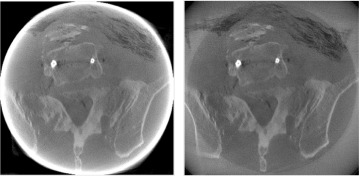
Left: No correction. Right: Projection extrapolation and extended FOV with multi-resolution.
This correction is a bit more complicated than the others as there isn’t a single option to turn on. There are two main options: projection extrapolation and extended FOV. For projection extrapolation, the projection images
can be extrapolated in the transaxial and/or axial directions, essentially top/bottom and left/right. The default extrapolation length is 25% (0.25) of the original size per direction (so a total of 1.5 increase in size), but this can be optionally adjusted with
options.extrapLength. This is, however, a global adjustment so it adjust both the transaxial and axial directions. You can specify a more specific extrapolation lengths with options.extrapLengthTransaxial and options.extrapLengthAxial.
If you specify one, but not the other, and you have chosen both extrapolation directions, then the default value of 0.25 is used.
The extrapolation is a simple next/previous extrapolation, i.e. depending on the side, either the previous or next value is used (i.e. the border value is reused). The extrapolated data can also be optionally scaled logarithmically so that the very edge is air and the values scale
towards this air value from the original value taken from the edge of the original projection. Note that this step involves linearization of the data and then transforming it back into Poisson-based count data, which can cause some numerical inaccuracy
in the extrapolated regions. Currently, this weighting is off by default, but you can enable it by setting options.useExtrapolationWeighting to true before the CTEFOVCorrection function is called. The original data is not affected by this.
You can separately select the transaxial and axial extrapolations with options.transaxialExtrapolation and options.axialExtrapolation, respectively. The extrapolation itself is enabled with
options.useExtrapolation.
In addition to, or alternatively, you can use extended FOV. This simply extends the FOV, but has some additional advantages over doing this manually. First, the image is automatically cropped to the original size, second,
regularization is generally only applied to the main FOV and third, you can select multi-resolution reconstruction. As with extrapolation, the extended FOV can be applied to the transaxial direction (XY) and/or the axial direction (Z) with
options.transaxialEFOV and options.axialEFOV, respectively. You can enable extended FOV with options.useEFOV. Normally, the extended FOV uses the same voxel size, but you can use increased voxel size with the multi-resolution
reconstruction, enabled with options.useMultiResolutionVolumes. The extended volume is divided into separate volumes, where the amount depends on whether transaxial and/or axial directions are included. If both are included, there
will be 6 multi-resolution volumes plus the main volume. The multi-resolution volumes can have a larger voxel size than the main volume. This can be controlled with options.multiResolutionScale, where the default value of 1/4 means
that the original size is divided by this value, i.e. the resolution is 1/4 of the original and the voxel size four times larger. The default extended FOV extension length is 40% (0.4) in transaxial direction of the original size per side (for a total of 1.8 times the original FOV).
For axial direction, by default the code tries to compute the optimal axial extension such that the X-ray cone is just within the volume (this also includes extrapolation if selected) but this requires that sourceToDetector and
sourceToCRot variables are present in the input class object (options). If these are not present, a default value of 30% (0.3) is used.
With 1/4 scale, this is essentially reduced to a 10% increase (transaxial) in voxel count. You can adjust this globally with options.eFOVLength or specifically with options.eFOVLengthTransaxial and options.eFOVLengthAxial.
Note that if options.eFOVLengthAxial is manually set, it is ALWAYS used. With multi-resolution volumes, the mask image and regularization are only used for the main volume!
See https://doi.org/10.1088/1361-6560/aa52b8 for details on the multi-resolution method. Note that the OMEGA implementation does not match the paper.
See https://dx.doi.org/10.1118/1.1776673 for another example of projection extrapolation.
Multi-resolution
It is possible to use multi-resolution reconstruction without any extended FOV. However, this requires you to use a smaller “effective” FOV and then extend the FOV to the original size using options.eFOVLength (or specific values for transaxial and axial).
Note that by default the image volume is always cropped to the “effective” FOV. To save the multi-resolution volumes, you need to set CELL to true in:
https://github.com/villekf/OMEGA/blob/master/source/cpp/structs.h#L10 and recompile the files. This outputs a cell matrix in MATLAB/Octave. The first element is the main volume. For Python, you also need to set options.storeMultiResolution = True before
reconstruction in addition to the above. The image is then output as a vector that contains all the volumes in one vector. You need to manually separate them.
This is currently not possible automatically, but it is possible to have specific volumes in specific regions, i.e. the main volume may not be the center volume. This requires modifying https://github.com/villekf/OMEGA/blob/master/source/m-files/setUpCorrections.m
and https://github.com/villekf/OMEGA/blob/master/source/m-files/computePixelSize.m. Especially important are the correct FOV sizes, number of voxels per volume, and the bx/y/z values, which correspond to the edges where the volumes begin.
The reconstruction process should work fine as long as these values are correctly adjusted.
When using built-in algorithms, not all algorithms support multi-resolution reconstruction. Unsupported algorithms are CGLS and LSQR. Some other algorithms also might not work optimally with multi-resolution reconstruction.
Note
This feature works similarly whether using built-in algorithms or custom algorithms with the projector operators. For the projector operators, the process is somewhat more complex. See the CBCT examples for more details on how to perform multi-resolution reconstruction.
Offset correction
This is a CT-only feature and can be enabled with options.offsetCorrection. If you have an offset imaging case, i.e. the center of rotation is not at the origin, setting this to true should remove any offset artifacts. This is often called redundancy weighting.
The weighting should be done automatically.
Examples of offset papers include https://dx.doi.org/10.1109/nssmic.2010.5874179 https://dx.doi.org/10.1088/0031-9155/58/2/205 and https://dx.doi.org/10.1118/1.1489043 and https://dx.doi.org/10.1088/1361-6560/ac16bc. Note that although they present different weights, the results are the same.
Note
This feature works the same way whether you are using built-in algorithms or custom algorithms with the projector operators.
Resolution recovery
In SPECT, modeling the response of the collimator is commonly referred to as resolution recovery. Also known as collimator-detector response correction, full modeling of the collimator includes considering the geometry of the collimator, septal penetration, and collimator
scatter. However, the built-in resolution recovery in OMEGA accounts only for the geometrical response, which is the most significant component in the collimator-detector response. Thus, this is a SPECT-only feature, and is supported by projector models 1, 2, and 6. Resolution recovery
parameters can be determined automatically using the collimator dimensions or manually by setting the relevant variables. The geometry of the collimator is input into the variables options.colL, options.colR, options.colD, options.colFxy, and options.colFz. These
define the hole length, radius, separation from detector surface, focal distance in the XY (transaxial) direction, and focal distance in Z (axial) direction, respectively. Currently, focal distances of zero and Inf are supported, representing pinhole and parallel-hole collimators, respectively.
With projector type 1, resolution recovery is performed by tracing multiple rays for each detector pixel/data point. The collimator is modeled by the relative shifts of the traced rays. The shifts for each detector element can be entered into the variables options.rayShiftsSource
and options.rayShiftsDetector. The former encodes the shifts at the detector-collimator interface, and the latter encodes the shifts at the middle of the collimator. The variables should be of the size 2*options.nRays * options.nRowsD * options.nColsD * options.nProjections,
with the elements [x0, y0, x1, y1] depicting the shifts in the detector coordinate system in millimeters.
The orthogonal distance ray tracer weighs voxels by a Gaussian distribution, the variance of which is defined by the variables options.coneOfResponseStdCoeffA, options.coneOfResponseStdCoeffB, and options.coneOfResponseStdCoeffC. The characters A, B, and C refer to the
collimator-detector response model, where the Gaussian FWHM is sqrt((az+b)^2+c^2), z being the distance along the normal vector of the detector element.
Projector type 6, the rotate-and-sum method, considers the detector response by convolving the image volume with options.gFilter during projection.